On this page
Waves, frequency, and wavelength
An alternating current in a conductor produces a changing electric and magnetic field around it. When the current alternates fast enough, that field detaches from the conductor and propagates as an electromagnetic wave. The wave is described by three quantities. The cycle is one complete oscillation of the field. The amplitude is the peak strength of the field, measured from the zero line to the crest. The frequency is the number of cycles per second, measured in hertz (Hz): one cycle per second is 1 Hz, a thousand is 1 kHz, a million is 1 MHz, a billion is 1 GHz.1
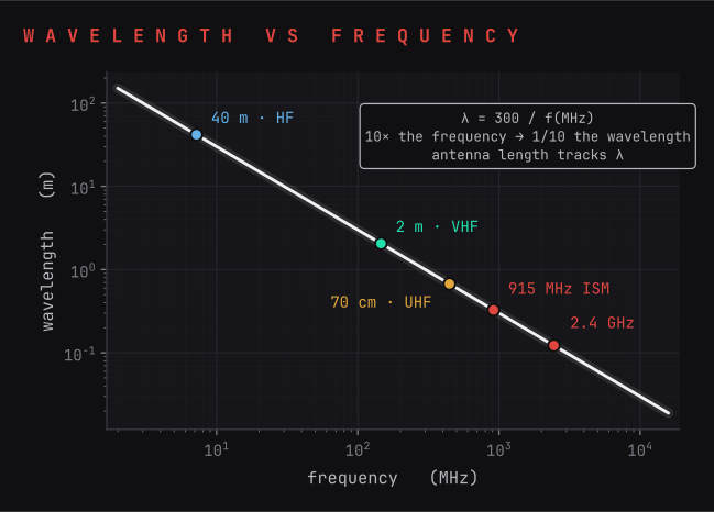
The wavelength is the distance one cycle occupies in space. Because every radio wave travels at the speed of light, c = 299,792,458 m/s (taken as 3 × 10⁸ m/s for field work), frequency and wavelength are fixed by a single equation:
With frequency in MHz this reduces to the field form: “In order to find wavelength in meters, divide 300 by the frequency in MHz.”1 The relationship is inverse, so higher frequencies are physically shorter: 3.9 MHz is 77 m, 7.2 MHz is 42 m, 146 MHz is 2.05 m, 446 MHz is 0.67 m, 915 MHz is 0.33 m, and 2450 MHz is 0.122 m.3 Wavelength governs the rest of the module: it sets the resonant length of an antenna (Unit 06), the size of obstacle a wave diffracts around (Unit 05), and how readily a signal passes through a wall (Unit 02).
A whole-number multiple of a frequency is a harmonic: “A frequency that is twice as great as the fundamental frequency is called the second harmonic; a frequency three times as great is the third harmonic.”11 Harmonics matter in two ways: a transmitter radiates unwanted energy at them, and one antenna cut for a low band can be reused on a band three times higher, because it is resonant at that harmonic.4
The spectrum and its bands
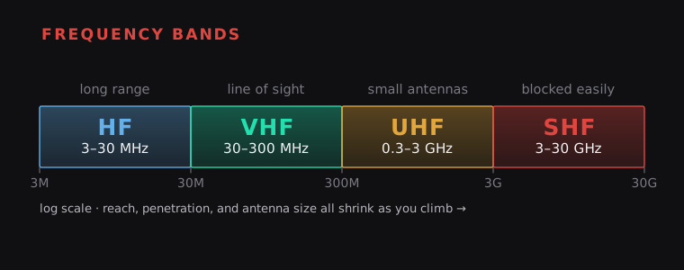
The spectrum is divided into bands by decade of frequency. Each band has a characteristic propagation behavior that follows directly from its wavelength, and those behaviors, not preference, decide which band a given task uses.1
HF, 3 to 30 MHz, is primarily propagated as sky waves: the signal refracts off the ionosphere and returns to earth, traveling long distances at low power, and ranges of hundreds to thousands of miles are routine, though temperature and humidity along the path can degrade the signal.1 VHF, 30 to 300 MHz, is used for mobile two-way communication; it is more susceptible to attenuation than HF, so line-of-sight propagation is imperative, and the signal is extended beyond line of sight only by troposcatter, satellites, and repeaters.1 UHF, 300 MHz to 3 GHz, is used for line-of-sight communications and can take advantage of ducting; its common applications are GPS, cellular communications, and wireless LAN.1 SHF, 3 to 30 GHz, is used for radar, satellite communications, wireless LAN, and microwave relay links, typically through high-gain, highly directional antennas.1
Three quantities move together as frequency rises: range shortens, penetration through structures worsens, and antenna size shrinks. A doctrinal reference tabulates the range trade directly: HF gives 0–50 miles by ground wave and 100–8000 miles by sky wave; VHF gives 0–30 miles ground and 50–150 miles sky; UHF gives 0–50 miles and is essentially line-of-sight only.4 Antenna size follows wavelength from Unit 01: a half-wave HF antenna is tens of meters of wire, while a half-wave element at 915 MHz is 16 cm.
In the United States every frequency is allocated to a service, and the allocation determines who may transmit there and under what rules. The amateur bands are the lawful place to practice transmitting most of what this module covers. Under 47 CFR Part 97, transmitting on an amateur band requires an FCC license: the station apparatus must be under the physical control of a person named in an amateur station license grant.12 There are three license classes: Technician (entry level, privileges on all bands above 30 MHz plus limited HF), General (privileges on all amateur bands), and Amateur Extra (all privileges on all bands and modes).7 Receiving is not licensed: listening, modeling, cutting antennas, and surveying the spectrum transmit nothing and require no license.
Power and decibels
Radio power spans from tens of watts at a transmitter down to a fraction of a picowatt at a receiver, ten or more orders of magnitude. The decibel expresses that range as a logarithm, which turns multiplication into addition: a chain of gains and losses becomes a single sum. Three forms are used, and mixing them is the most common beginner error. dB is a dimensionless ratio between two powers, dB = 10 log₁₀(P₂/P₁); it expresses a gain or a loss, not an amount.1 dBm is an absolute power referenced to 1 milliwatt, so it names an actual amount: 0 dBm is 1 mW and 30 dBm is 1 W.1 dBi is antenna gain referenced to an isotropic radiator, a theoretical antenna that radiates equally in all directions.3
Power is converted to dBm in the field by the rule of 3 and 10, starting from 1 W = 30 dBm: doubling power adds 3 dB, halving subtracts 3 dB; multiplying by 10 adds 10 dB, dividing by 10 subtracts 10 dB.11 The full conversion, tabulated from the 1 W baseline:
| Power | dBm | Power | dBm |
|---|---|---|---|
| 0.125 W | 21 | 4 W | 36 |
| 0.25 W | 24 | 5 W | 37 |
| 0.5 W | 27 | 10 W | 40 |
| 1 W | 30 | 100 W | 50 |
| 2 W | 33 | 1000 W | 60 |
Worked the other way: convert 25 mW by chaining the two rules. Start at 100 mW, which is one tenfold step below 1 W (30 dBm), so 100 mW is 20 dBm. Halve it twice: 50 mW is 20 minus 3, or 17 dBm, and 25 mW is 17 minus 3, or 14 dBm. Once every term is in dBm and dB, an entire link is one addition, which is the subject of Unit 04.
Free-space path loss and the horizon
A wave radiated into free space spreads over the surface of an expanding sphere, so the power crossing a fixed receiving aperture falls with the square of distance. Expressed in decibels, this is free-space path loss (FSPL), the loss between two antennas with an unobstructed path and no obstacles in the Fresnel zone (Unit 05). The standard engineering form is:
Both distance terms are 20 log₁₀, which produces the two rules that do most of the planning work. Doubling the distance adds 20 log₁₀(2) = 6 dB. Doubling the frequency adds the same 6 dB. Across a decade of frequency the effect is large: at equal distance, 2450 MHz loses 20 log₁₀(2450/146) = 24.5 dB more than 146 MHz. The plotted curves show both axes at once.
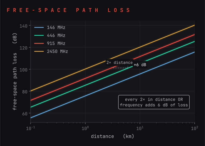
A worked example fixes the scale. A 900 MHz signal over an 8 km free-space path loses 32 + 20 log₁₀(900) + 20 log₁₀(8) = 109.14 dB.14 One watt (30 dBm) into that path arrives at −79 dBm before antenna gain, still well above a receiver's sensitivity: low power spans real distance when the path is clear.
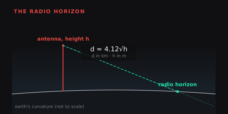
Free space ends at the horizon. VHF and above travel in nearly straight lines while the earth curves away, so a line-of-sight link's reach is set by antenna height, not power. Atmospheric refraction bends the wave slightly downward, extending the radio horizon about 15% past the visual one:
When the far end sits beyond that sum, the options are a taller mast, a relay between, or a different propagation mode: HF sky wave over the top (Unit 05), or a satellite, whose line-of-sight horizon from orbit already covers a continent.
Put the decibel arithmetic and the path loss together and you have the link budget: transmit power, minus feedline loss, plus antenna gains, minus path loss, compared against the receiver's sensitivity.3 Work the sum yourself below; the presets are the series' own links.
Real-world propagation
Free space is the best case; a real path is always worse, and the wave reaches the receiver by one of three mechanisms.14 A ground wave (the surface wave plus a ground-reflected wave) follows the earth's curvature and dominates at low frequencies. A space wave (also called the direct wave) is the line-of-sight path of Unit 04. A sky wave radiates upward, refracts off the ionosphere, and returns to earth far away.
The ionosphere is the band of the upper atmosphere that solar radiation ionizes into free electrons, in layers at characteristic altitudes.5 The D layer, 30 to 55 miles up, refracts only low frequencies and absorbs HF, passing it through with attenuation, and it disappears after sunset. The E layer, 55 to 90 miles, refracts frequencies up to about 20 MHz and is useful for ranges to about 1500 miles. The F layer, 90 to 240 miles, splits into F1 and F2 in daylight and merges at night, and it is responsible for most HF long-distance transmission.5
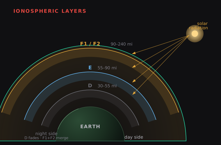
Because the layers' ionization changes with the sun, the usable frequency band changes with it. Three limits bound it. The maximum usable frequency (MUF) is the highest frequency the ionosphere will still refract back to earth on a given path; above the MUF the wave passes into space. It is highest around local noon. The lowest usable frequency (LUF) is set by D-layer absorption below. Between them, the frequency of optimum transmission (FOT) is the working choice, approximately 85% of the MUF.515
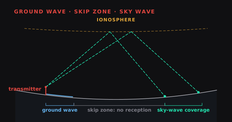
Between the end of ground-wave range and the first sky-wave return lies the skip zone, a ring that receives neither wave. Under ideal conditions the ground wave fails at about 50 miles, and frequency or antenna choice can leave a skip zone of 50 to 70 miles.16
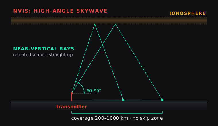
NVIS (near-vertical incidence sky wave) closes the skip zone. High-angle antennas radiate HF almost straight up, at take-off angles above 60 degrees, and the ionosphere reflects it back down over a wide circle: “Because of the near-vertical radiation angle, there is no skip zone.”14 The usable band is narrow and follows the ionosphere: 2 to 4 MHz at night, 4 to 8 MHz by day.16 Coverage radius runs from 200 to 1000 km, filling exactly the regional gap that neither line-of-sight nor long-hop sky wave reaches.16 The one antenna decision that produces it is height, covered in Unit 06.
Waves also reflect, diffract around edges, scatter, and are absorbed. Diffraction loss is severe: a signal may lose 30 to 40 dB by being bent only 5 feet by a mountain ridge.14 Multiple copies arriving by different paths interfere, which is multipath. The urban environment produces all of these at once: walls reflect and absorb, and absorption through a structure rises with frequency, so a UHF signal that passes a wall easily may be blocked at 5 GHz.1
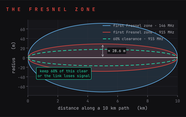
Line-of-sight links carry a further requirement. The wave needs a clear ellipsoid of space around the sight line, the first Fresnel zone; a common engineering rule requires 60% of its radius clear, while the doctrinal rule of thumb states the maximum obstruction allowable is 40% and the recommended obstruction is 20% or less.314 The zone radius at midpath is r = 8.657 √(d / f), with r in meters, d the path length in km, and f in GHz: over a 2 km path, that is 12.8 m at 915 MHz but only 5.0 m at 5.8 GHz.17 Obstacles inside the zone diffract and cost signal even when the far antenna is plainly visible.
Terrain sums all of these losses, and the total can dwarf free space. The reference model for computing it is Longley-Rice, the Irregular Terrain Model. Anita Longley and Phil Rice of the Institute for Telecommunication Sciences published it in 1968 to predict radio loss over irregular terrain. It covers 20 MHz to 20 GHz and still runs inside today's commercial coverage tools.8 The open-source implementations SPLAT! and Signal Server run it locally against free elevation data.910
Antennas and feedlines
An antenna is a conductor cut to resonate at the wavelength it radiates. The reference is the half-wave dipole: two equal legs fed at the center, a half wavelength end to end. Its length is cut by formula, which already includes the roughly 5% shortening real wire needs relative to the free-space half wavelength:4
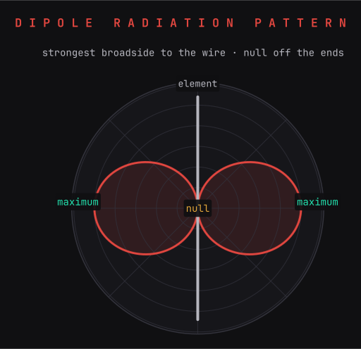
Worked at 7.2 MHz: 468 / 7.2 = 65 feet total, so each leg is 32.5 feet. The half-wave dipole is horizontally polarized, handles high power, radiates bidirectionally broadside to the wire, and is resonant within about ±2% of its design frequency; outside that band the match degrades.4 Its gain is 2.14 dBi, the reference point against which other antennas' gain in dBi is measured.18
Height controls the take-off angle, which is what Unit 05 called for. A horizontal dipole between 0.1 and 0.25 wavelength above ground radiates most of its energy at high angles: this is the NVIS configuration.16 Raised toward a half wavelength and higher, the pattern lowers toward the horizon for long-distance work. The height formulas follow the same form as the length:4 quarter-wave height = 246 / f (feet), half-wave height = 492 / f (feet).
Two variations cover most field cases. A quarter-wave vertical is half a dipole stood on end, worked against a ground plane or radials, radiating omnidirectionally in azimuth with vertical polarization. An inverted V is a dipole hung from a single central support with the ends sloping down; it needs only one mast, produces combined horizontal and vertical polarization, and has slightly less gain than a flat dipole.4
Every antenna has a radiation pattern, identical on transmit and receive: the dipole is strongest broadside to the wire and has deep nulls off its ends. Pointing an end at the far station points the null.
Polarization is the orientation of the wave's electric field, fixed by the transmitting antenna. Matching it matters: a receiving antenna cross-polarized (90 degrees) to the incoming wave loses on the order of 30 dB, a larger loss than most link budgets can absorb.3 The choice is partly set by band. At MF and LF, ground-wave propagation requires vertical polarization; at HF with sky wave it makes little practical difference; at VHF and UHF either works, though below about 50 MHz a vertical gives a stronger signal for a low, vehicle-height antenna.14
Between radio and antenna sits the feedline, and the antenna must present a load it can carry. SWR (standing wave ratio) measures the match: 1:1 is ideal, 1.5 to 2 is acceptable, 2 to 3 is workable with noticeable loss, and 3:1 or higher is a fault to correct.3 A mismatch reflects power back toward the transmitter; the coax itself also loses energy to conductor resistance and dielectric loss on every meter, and that loss rises with frequency. The vault's field references give it only qualitatively: 10 to 20 dB of loss is not unusual in a 30 meter run of coax at higher frequencies.19 Trimming an antenna to lowest SWR at the operating frequency is the practical procedure: cut the legs slightly long, measure SWR, and shorten by the same percentage the frequency needs to rise.20 Salvaged whips, antennas, and coax from discarded electronics are cut-to-length raw material for all of it.
Work the full decision below: band, expedient antenna type, cut length, and siting, with the NVIS height effect from Unit 05 built in.
Receivers and the noise floor
Two specifications define a receiver. Sensitivity is the weakest signal it can turn into usable output; selectivity is its ability to accept one signal while rejecting adjacent ones.2 Sensitivity is not arbitrary: it is bounded from below by the noise the receiver itself and the antenna deliver. The floor is thermal noise, kTB; sensitivity for any receiver is:
The equation shows the module's central point: sensitivity depends on bandwidth (B). Halving the bandwidth admitted lowers the noise floor by 3 dB, which is why the narrowband modes of Unit 08 are received where wideband modes are not, at equal power.
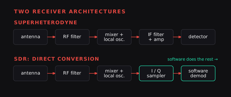
The architecture that delivers sensitivity and selectivity is the superheterodyne: mix the incoming signal with a local oscillator to a fixed intermediate frequency (IF), where one well-made filter does the selecting for any tuned frequency.2 A software-defined radio (SDR) keeps the front end but mixes down to two outputs 90 degrees apart, the in-phase (I) and quadrature (Q) branches, digitizes them, and does all filtering and demodulation in software.21 The bandwidth an SDR can show at once equals its sample rate: a receiver sampling at 2.4 million samples per second shows 2.4 MHz of spectrum at a time.21
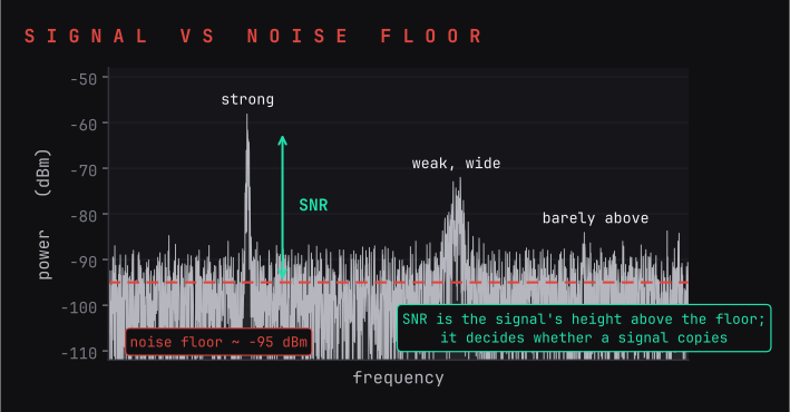
The noise floor is the level of ever-present radio noise (thermal plus man-made) below which an ordinary receiver cannot recover a signal. Its makeup changes with frequency: atmospheric noise dominates from 0 to 5 MHz, and galactic noise dominates above that.14 What decides a link is never received power alone but the signal-to-noise ratio (SNR), the height of the signal above the floor. A waterfall display shows the floor as the speckled background and each signal as a stripe standing out of it; on an SDR the operator sets the display's lower limit to the floor to see intermittent signals emerge.22
Modulation and bandwidth
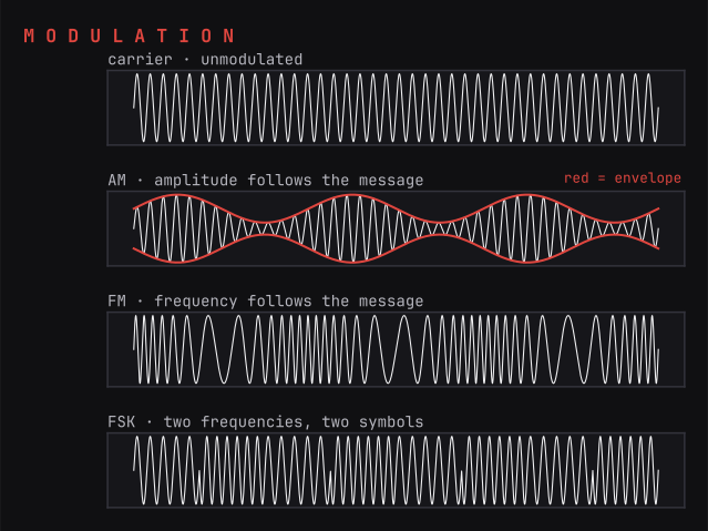
A carrier wave conveys nothing until one of its properties is varied with a message: that variation is modulation. The three analog forms vary the three properties of the wave. Amplitude modulation (AM) varies the carrier's strength. Its weakness is efficiency: at least two thirds of the transmitted power sits in the carrier itself, which carries no information.14 Single sideband (SSB) removes the carrier and one sideband, making it about three times more power-efficient than AM for the same voice and occupying less bandwidth.14 Frequency modulation (FM) varies the carrier's frequency and is more robust against amplitude fading, at the cost of wider bandwidth.14 A course reference gives the trade in plain terms: AM has a “relatively small bandwidth 6 KHz,” so “less information is able to be imposed on signal,” while FM's “wider bandwidth” enables “more information to be imposed on carrier frequency” but “requires more use of the radio spectrum to operate.”30
Digital modes shift the carrier between discrete states: FSK (frequency-shift keying) switches between frequencies, PSK (phase-shift keying) between phase positions, ASK between amplitudes.14 Trunked digital voice systems (P25, DMR, NXDN) build on these; DMR, for example, places two time-division slots on one 12.5 kHz channel, so one channel carries two conversations.23
Bandwidth is where modulation meets the noise floor of Unit 07. From the sensitivity equation, noise power is proportional to bandwidth, so a narrower mode competes against less noise and is received at lower power. Occupied bandwidth spans four orders of magnitude across common modes:
| Mode | Occupied bandwidth |
|---|---|
| Analog fast-scan TV | ~6 MHz |
| FM voice (VHF repeater) | 10–15 kHz |
| DMR digital voice | 12.5 kHz (two slots) |
| SSB voice | ~3 kHz |
| CW (Morse) | ~150 Hz |
| PSK31 (keyboard) | ~31 Hz |
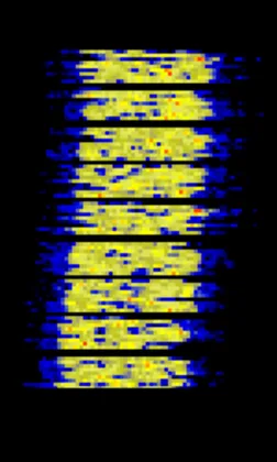
≈50 Hz
GFSK
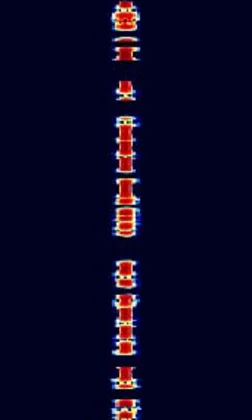
≈150 Hz
OOK
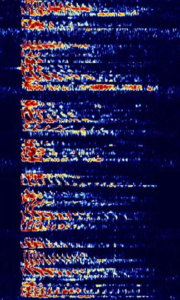
≈1.9 kHz
SSB
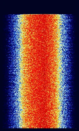
12.5 kHz
FSK
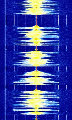
12.5 kHz
C4FM
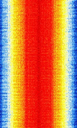
≈180 kHz
WFM
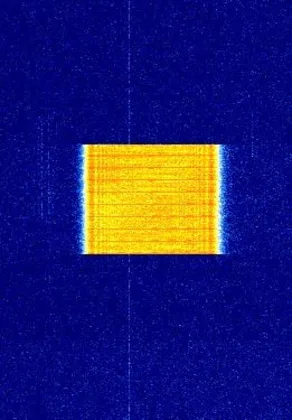
≈250 kHz
CSS
This is the physics behind narrowband digital modes at low power. PSK31 is 31 baud in about 31 Hz;2 keyboard modes like JS8 trade speed for sensitivity, decoding signals more than 20 dB below the noise in a 2.5 kHz reference bandwidth at their slowest settings.24 The low-power bearer radios that carry Reticulum traffic sit at this same end of the trade, exchanging data rate for range at milliwatt powers.
The same physics governs emission control. Every transmission reaches every receiver in range, including a direction-finding (DF) receiver: strong signals travel farther, all the way to an adversary's DF receivers, and raising power to overcome jamming raises DF vulnerability at the same time.6 DF turns a signal into a location. A single bearing is a line of bearing; two crossed bearings are a cut; three are a fix.25 Practical DF systems are accurate to about 2.5 degrees RMS for a basic amplitude-comparison set and about 1 degree for a calibrated interferometer;13 at 100 km, two ideal 1-degree sites bracket an emitter to a circle roughly 2 km across.13 Two properties are worth separating. A low probability of intercept (LPI), which spread-spectrum modes achieve by lowering the signal below the noise, is not a low probability of detection: spread-spectrum techniques can reduce the apparent SNR by 20 to 40 dB, but a constant emitter is still locatable.13 The three levers the operator controls are power, antenna pattern, and airtime. Applying them is a later module's subject.
Field exercise
The module explained the spectrum; the exercise is to listen to it. With a free, open-source software-defined radio you can tune from the broadcast bands through the amateur bands and hear the module's ideas directly, recognizing each modulation by its sound and by its shape on the waterfall. The receiver's spectrum display shows signal strength across frequency right now; its waterfall shows the same over time, so intermittent signals leave a trail and a Morse signal's dots and dashes draw tracks.22
Task: Using an open-source SDR, tune across the spectrum and learn to recognize the common bands and the common modulations by ear and by their waterfall signature.
Condition: Given a computer running SDR++, a free, open-source (GPL-3.0), cross-platform application for Windows, macOS, and Linux,22 with a low-cost RTL-SDR receiver (about $25, tuning roughly 29 to 1700 MHz and showing up to 2.4 MHz of spectrum at once)21 and an antenna; or, with no hardware, a public WebSDR in a browser. The AM broadcast band and the HF amateur bands in the Standard sit below that dongle's tuning range: reach them with a receiver that covers HF, or use the WebSDR for those bands. Work receive-only: the Electronic Communications Privacy Act bars intercepting mobile phone and pager traffic, so stay on broadcast, amateur, and utility signals.21
Standard: The receiver tuned across at least three bands: the AM broadcast band (530 to 1700 kHz),28 the FM broadcast band (87 to 108 MHz),22 and an HF amateur band (40 meters, 7.000 to 7.300 MHz, or 20 meters, 14.000 to 14.350 MHz).7 At least five signals found and logged by frequency, band, and the SDR++ demodulator that copies each (AM, WFM, USB or LSB, CW).22 At least four modulation types recognized by ear and by waterfall shape: AM (a carrier flanked by two sidebands), FM broadcast (a wide block about 150 kHz across), SSB voice (a narrow trace about 3 kHz wide with no carrier, upper sideband above 10 MHz and lower sideband below),22 CW (on-off Morse tones, the narrowest signals on the band, drawing dot-and-dash tracks on the waterfall), and one digital mode: FT8, which appears as repeating traces about 50 Hz wide on a fixed cycle near 7.074 or 14.074 MHz,28 or PSK31, a line about 31 Hz wide near 7.040 or 14.070 MHz.282 For each signal, the band named with why it suits that traffic (Unit 02) and its bandwidth compared with the others on the waterfall (Unit 08). Any unknown signal run against the Signal Identification Wiki's waterfall and audio references.21
Module test
Task: Complete the Module 06 test.
Condition: Given ten questions covering units one through eight, without reference to the module units or notes.
Standard: Answer at least eight of ten questions correctly. For each question missed, reread the unit named in the feedback and retake the test until the standard is met.
Key formulas
Each formula is taught in the unit noted, next to its worked example. This card collects them for the field exercise and for working a link budget.
×2 = +3 dB ×10 = +10 dB
kTB = −174 dBm/Hz
Glossary
- dB
- Decibel: a logarithmic ratio between two power levels; gains are positive, losses negative.
- dBi
- Antenna gain relative to an ideal isotropic radiator.
- dBm
- Absolute power referenced to one milliwatt; 1 W equals 30 dBm.
- Dipole
- A two-legged, center-fed antenna a half wavelength long end to end.
- Free-space path loss
- The attenuation between two antennas over an unobstructed path, growing 6 dB per doubling of distance.
- Fresnel zone
- The ellipsoid of space around a sight line that must be substantially clear for a line-of-sight link to work; 60% of the first zone's radius is the clearance rule.
- Link budget
- The decibel sum of a link: transmit power, minus losses, plus gains, compared with receiver sensitivity.
- Multipath
- Interference between copies of one signal arriving by different paths.
- Noise floor
- The ambient level of radio noise a signal must exceed to be received.
- MUF / LUF / FOT
- Maximum and lowest usable frequencies for a sky-wave path, and the frequency of optimum transmission (about 85% of the MUF) between them.
- NVIS
- Near-vertical incidence sky wave: high-angle HF propagation (take-off above 60 degrees) that returns from the ionosphere over a 200 to 1000 km circle around the transmitter, with no skip zone.
- Polarization
- The orientation of a wave's electric field, set by the transmitting antenna's orientation.
- Radiation pattern
- The directional distribution of an antenna's radiated or received energy.
- Radio horizon
- The distance at which a line-of-sight path grazes the earth's curvature; set by antenna height.
- Selectivity
- A receiver's ability to accept one signal while rejecting adjacent ones.
- Sensitivity
- The weakest signal a receiver can make useful, quoted in dBm.
- Skip zone
- The silent ring between the end of ground-wave range and the first skywave return.
- SNR
- Signal-to-noise ratio: the height of a signal above the noise floor, which decides whether it copies.
- SWR
- Standing wave ratio: the measure of mismatch between antenna and feedline; 1:1 is ideal.
Sources
- “Appendix A: RF Basics,” VHF/UHF communications reference (Light Fighter Library, Communicate/VHF-UHF). Band table and propagation characteristics; wavelength rule; dB and dBm definitions; free-space and non-free-space path-loss tables; reflection, refraction, diffraction, scatter, multipath, absorption definitions.
- Dan Romanchik KB6NU, The No Nonsense Technician Class License Study Guide, 2018 ed. (Light Fighter Library, Communicate/Radio). Receiver sensitivity and selectivity, superheterodyne architecture, mode bandwidth comparison (SSB ~3 kHz, FM 10–15 kHz, fast-scan TV ~6 MHz, CW ~150 Hz, PSK31 ~31 Hz).
- “Electromagnetic Waves, Radio Waves, and Antennas” primer (Light Fighter Library, Communicate/Radio). dBi definition; Fresnel-zone 60% clearance rule; SWR grading table (1:1 ideal, 1.5–2 acceptable, 2–3 workable, ≥3 poor); polarization and the ~30 dB cross-polarization loss.
- U.S. Marine Corps, MCRP 8-10B.11 Antenna Handbook (Light Fighter Library, Communicate/Antennas). Half-wave dipole length formula (“142 meters / Frequency in MHz or 468 feet / Frequency in MHz”) and height formulas (¼λ = 246/f ft, ½λ = 492/f ft); dipole and inverted-vee characteristics (±2% bandwidth, horizontal polarization, 1000 W); NVIS employment; radiation patterns.
- U.S. Army, TC 9-64 Communications-Electronics Fundamentals: Wave Propagation, Transmission Lines, and Antennas (Light Fighter Library, Communicate/Antennas). Ionospheric D/E/F layer altitudes (D 30–55 mi, E 55–90 mi, F 90–240 mi) and day/night behavior; critical frequency, MUF/LUF/FOT; skip distance and skip zone; Figures 2-14 and 2-19 (reproduced). Public domain (U.S. Government work).
- “Signature Management EPEMCON SOP: A Guide to Reduce Technical Signature” (Light Fighter Library, Communicate/EW-SIGINT). Reduce-power doctrine (“Strong signals travel farther—all the way to the adversary’s DF receivers”); the LPI versus LPD distinction; omnidirectional versus directional antenna exposure.
- ARRL, “Frequency Allocations” (US amateur band chart), arrl.org/frequency-allocations, and “Getting Licensed” (Technician, General, Amateur Extra classes), arrl.org/getting-licensed. Accessed 2026-07-23.
- NTIA Institute for Telecommunication Sciences, “Irregular Terrain Model (ITM) (Longley-Rice) (20 MHz – 20 GHz),” its.ntia.gov/software/itm (accessed 2026-07-23). Anita Longley and Phil Rice, 1968; 20 MHz to 20 GHz.
- John A. Magliacane KD2BD, SPLAT! (RF Signal Propagation, Loss, And Terrain analysis tool), open source; maintained fork at github.com/hoche/splat (accessed 2026-07-23).
- Signal Server, GPLv2 SPLAT!-derived RF simulator; maintained fork at github.com/W3AXL/Signal-Server (accessed 2026-07-23).
- “RF Theory Read Ahead: Fundamentals of Electricity” (Light Fighter Library, Communicate/EW-SIGINT). Wave anatomy (cycle, amplitude, frequency); harmonics; the rule of 3 and 10 and the watt-to-dBm conversion table (0.125 W = 21 dBm … 1000 W = 60 dBm).
- FCC, 47 CFR § 97.5, “Station license required,” via GPO govinfo (CFR 2023, Title 47): “The station apparatus must be under the physical control of a person named in an amateur station license grant.” Accessed 2026-07-23.
- David L. Adamy, EW 103: Tactical Battlefield Communications Electronic Warfare (Artech House). Free-space loss L = 32.44 + 20 log(d km) + 20 log(f MHz); receiver sensitivity S = kTB + NF + SNR, kTB = −174 dBm/Hz; DF accuracy (Watson-Watt ~2.5° RMS, interferometer ~1° RMS) and the CEP relationship (two 1° sites at 100 km → ~2 km CEP); spread-spectrum SNR reduction of 20–40 dB. Worked textbook examples (Light Fighter Library, Communicate/EW-SIGINT).
- “Electronic Warfare Fundamentals Student Guide, Volume I: Radio Fundamentals” (Light Fighter Library, Communicate/EW-SIGINT). Free-space loss worked example (900 MHz, 8 km = 109.14 dB); ground/space/sky wave taxonomy; NVIS defined (60–90° take-off, no skip zone); polarization by band; diffraction loss (30–40 dB over a 5-foot ridge); atmospheric noise dominant 0–5 MHz, galactic above; AM carrier inefficiency (≥⅔ of power in the carrier), SSB, FM, and FSK/PSK/ASK definitions.
- “RSLC Radio Wave Propagation” training deck (Light Fighter Library, Communicate/HF). FOT is approximately 85% of the MUF; daytime 10–20 MHz, nighttime 3–8 MHz long-haul.
- David M. Fiedler and Edward J. Farmer, Near Vertical Incidence Skywave Communication: Theory, Techniques, and Validation (1996; 2nd printing 2000) (Light Fighter Library, Communicate/HF). NVIS operating band (2–4 MHz night, 4–8 MHz day); coverage radius 200–1000 km; optimum dipole height 0.1–0.25λ; skip zone of 50–70 miles without NVIS.
- “DORA + CloudRF Engineer Mode Field Guide” (Light Fighter Library, Communicate/HF). Midpoint first-Fresnel-zone radius r(m) ≈ 8.657 √(d km / f GHz), with worked values at 915 MHz, 2.4 GHz, and 5.8 GHz.
- Joint Spectrum Center, Field Antenna Handbook (Light Fighter Library, Communicate/Antennas). Half-wave dipole gain of 2.14 dBi over isotropic; take-off angle by application (high for NVIS, low for long distance).
- U.S. Marine Corps, MCRP 6-22D Field Antenna Handbook (transmission-line loss, qualitative: “10 to 20 dB loss is not uncommon in a 30 meter length”), with quantitative reference from Times Microwave LMR-400 datasheet (1.5 / 2.7 / 3.9 dB per 100 ft at 150 / 450 / 900 MHz), timesmicrowave.com (accessed 2026-07-23).
- “A Field Guide to Simple HF Dipoles” (Light Fighter Library, Communicate/Antennas). The 95% length factor and the SWR trimming procedure (cut long, measure, shorten by the percentage the frequency must rise).
- Noah Axon, “Introduction to Software Defined Radio Supplement” (Light Fighter Homefront course material, 2024). I/Q (in-phase and quadrature) branches; sample rate equals shown bandwidth (2.4 MSPS → 2.4 MHz); superheterodyne and SDR block descriptions.
- “SDR++ User Guide” v1.1 (Light Fighter Library, LF-Course/Manuals). Waterfall display; setting the display floor to the noise floor to reveal intermittent signals; decimation and dynamic range.
- “DMR: An Introduction to Digital Mobile Radio” and “DMR Programming Workshop” (Light Fighter Library, Communicate). Two-slot TDMA on one 12.5 kHz channel carrying two simultaneous conversations.
- “JS8Call Guide” v2.2 (Light Fighter Library, LF-Course/Manuals). Mode speeds and decode thresholds: Slow (30 s frame, 25 Hz, decodes to −28 dB) through Turbo (6 s, 160 Hz, −18 dB).
- “Module 9: Direction Finding” (Light Fighter Library, Communicate/Direction-Finding). One line of bearing, two crossed bearings a “cut,” three a “fix”; baseline-length-to-depth rule of thumb.
- ITU-R Recommendation P.525-5, “Calculation of free-space attenuation” (11/2024), equation 6: Lbf = 32.4 + 20 log₁₀ f + 20 log₁₀ d dB, f in MHz, d in km. itu.int/rec/R-REC-P.525 (accessed 2026-07-23).
- “Line-of-sight propagation,” Wikipedia, en.wikipedia.org/wiki/Line-of-sight_propagation (accessed 2026-07-23). Geometric horizon “horizon_km ≈ 3.57 ⋅ √height_metres”; refracted horizon under the 4/3 k-factor “d ≈ 4.12 ⋅ √h for h in metres and d in kilometres”.
- Signal Identification Wiki, FT8 (50 Hz, repeating cyclic traces near 7.074 / 14.074 MHz) and PSK31 (~31 Hz, narrow stable lines near 7.040 / 14.070 MHz), accessed 2026-07-23. AM broadcast band 530–1700 kHz (10 kHz spacing) and FM broadcast band 87–108 MHz per the SDR++ demodulator reference (src 22) and standard US allocations. NOAA Weather Radio: seven channels 162.400–162.550 MHz, 25 kHz spacing, weather.gov/nwr.
- AresValley, Artemis signal-identification database (SigID DB v74, 2026-07-18; GPL-3), github.com/AresValley/Artemis-DB. Waterfall captures and the listed occupied bandwidth and modulation for JS8 (≈50 Hz, GFSK), single-sideband voice (≈1.9 kHz), DMR and P25 (12.5 kHz), FM broadcast (WFM), and LoRa (≈250 kHz, CSS). The database carries the records of the Signal Identification Wiki (src 21); each capture is reproduced from its wiki entry.
- U.S. Army 18E SWC, Mr. Sharp Communication Book, Course Book 2 (Light Fighter Library, Communicate/Handbooks). Modulation is “the mixing of one signal onto another”; AM “changing the amplitude” with a “relatively small bandwidth 6 KHz”; FM “changing the frequency” with “wider bandwidth, enabling more information”; SSB “does not take up entire bandwidth”; CW a keyed “solid tone” turned “on and off at will” to form International Morse Code.